Richard Hu
Quantitative Technologist @ Radix Trading
How to Almost Find the SVD of a Matrix Really Fast
Posted on December 25, 2022
The singular value decomposition (SVD) has applications in compression, signal processing, natural language processing, quantum information, big data, numerical weather prediction, financial engineering, gravitational waveform modeling, disease surveillance, and recommender systems to name just a few.
It is one of the most important techniques in linear algebra, so much so that in 2000 (before some of the aforementioned applications even existed), it was named as part of the top 10 algorithms of the 20th century.
Unfortunately, as data has grown more abundant and matrices in applications have grown larger, the computation of the SVD has become increasingly challenging, leaving researchers searching for new methods to more efficiently perform possibly the most important matrix factorization.
In the end, they found an incredibly powerful solution capable of scaling up to the supermassive problems in computing today and saving orders’ of magnitudes worth of computational resources.
There’s just one critical caveat about it, though.
It gets the answer wrong.
Why Settle with Wrong? ⇱
Traditional, deterministic methods for computing the SVD of an \(m \times n\) matrix take \(\mathcal{O} \left( m^2 n + n^3 \right)\) time and also have a memory complexity superlinear in \(m\) and \(n\). We assume here that \(m \geq n\) because if that’s not the case, we can just compute the SVD of the transposed matrix.
For small matrices, this is no big deal but once \(m\) and \(n\) reach on the order of billions, the SVD becomes effectively intractable. So how can we do better?
A key insight is that structured, non-random matrices usually exhibit rapidly-decaying singular values. For example, consider this picture from one of my hikes in the Big Sur, rendered in grayscale.

Plotting the singular values yields a sharply-decreasing singular sprectrum. Notice the log-scale x-axis.
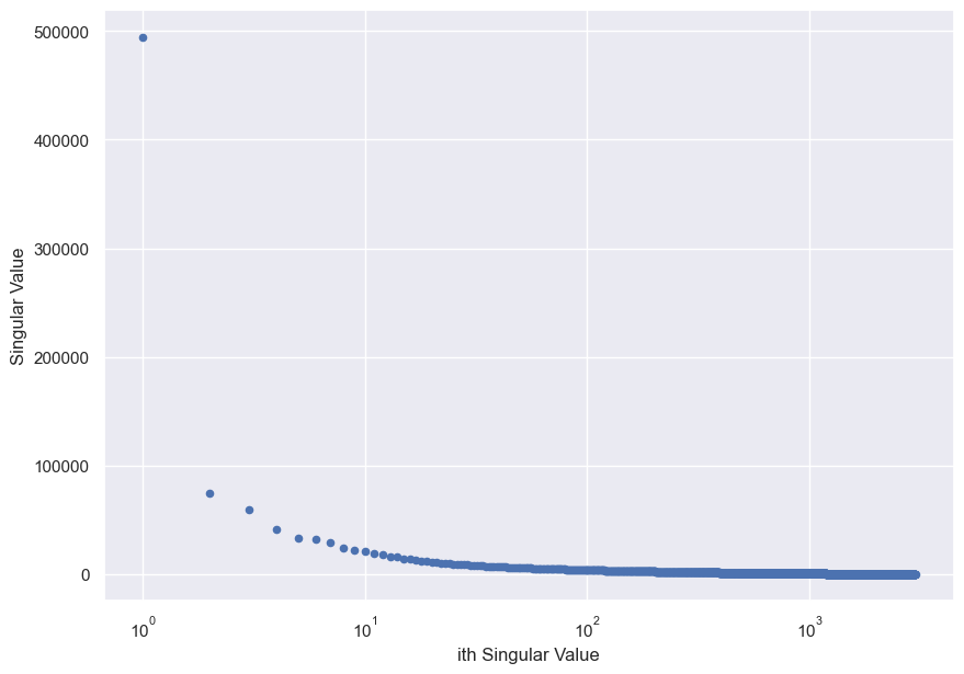
This behaviour occurs because often, structured data from the real world is an amalgamation of a few prominent features and little bits of noise (think Pareto principle).
We say such a matrix \(\mathbf A\) has a low numerical rank, and we can achieve an extremely accurate approximation of \(\mathbf A\) by taking its SVD and throwing out all but the top few singular values and singular vectors.
\[\underbrace{\mathbf A}_{m \times n} \quad \approx \quad \underbrace{\mathbf U}_{m \times k} \quad \times \quad \underbrace{\mathbf \Sigma}_{k \times k} \quad \times \quad \underbrace{\mathbf V^*}_{k \times n}\]Here, \(k\) is much smaller than the true rank \(A\) and this modified SVD is an example of a low-rank approximation. In addition to reducing storage footprints and speeding up matrix-matrix and matrix-vector multiplication, low-rank approximations are frequently used to solve computational problems like least squares and PDEs.
Thus, it is almost always the case in the real world that we are happy with just working with a low-rank approximation of our matrices, meaning that we no longer care about computing every single singular value and singular vector. This observation allows for astronomical reductions in the computational requirements of the SVD and forms the basis of most randomized numerical linear algebra (RandNLA) techniques.
A Slightly Inaccurate Algorithm for Computing the SVD ⇱
In 2009, Nathan Halko, Per-Gunnar Martinsson, and Joel A. Tropp published “Finding structure with randomness: Probabilistic algorithms for constructing approximate matrix decompositions,” which would prove to be a seminal paper in RandNLA. Observing that matrix factorizations like the SVD can be used to derive generalized methods for solving many computational problems, Halko et al. proposed a two-stage framework for efficiently computing the low-rank approximation of an \(m \times n\) matrix \(A\).
-
Find an orthonormal matrix \(\mathbf Q\) such that \(\mathbf A \approx \mathbf Q \mathbf Q^* \mathbf A\). \(\mathbf Q\) can be thought of as an approximate basis for \(\mathbf A\) and ideally, it should have as few columns as possible.
-
Use \(\mathbf Q\) to compute an approximate factorization of \(\mathbf A\).
We can utilize this framework to efficiently compute an approximate SVD of \(A\).
Algorithm: Approximate SVD
Given an orthonormal matrix \(\mathbf Q\) such that \(\mathbf A \approx \mathbf Q \mathbf Q^* \mathbf A\)
1. Compute the SVD of \(\mathbf Q^* \mathbf A\) using traditional, deterministic methods.
\[\mathbf Q^* \mathbf A = \mathbf U \mathbf \Sigma \mathbf V^*\]2. Return \(\mathbf Q \mathbf U, \mathbf \Sigma, \mathbf V^*\)
Observe that this algorithm does not produce a full SVD. For an \(m \times k\) matrix \(\mathbf Q\), this algorithm only gives us an approximation of the top \(k\) singular values of \(\mathbf A\) and their singular vectors.
However, it’s fast. A good choice of \(\mathbf Q\) results in \(\mathbf Q^* \mathbf A\) being very small, allowing for the deterministic SVD to run incredibly quickly.
Consequently, the chief problem is to efficiently form \(\mathbf Q\). Our desired \(\mathbf Q\) should satisfy a few properties: like mentioned before, it should have as few columns as possible and it should be orthonormal and moreover, its range should approximate the range of \(\mathbf A\), as we are ultimately trying to minimize the approximation error
\[\lVert \mathbf A - \mathbf Q \mathbf Q^* \mathbf A \rVert\]Halko et al. refer to this as the fixed-rank approximation problem, or just the fixed-rank problem for short, for a given \(k\).
We could trivially solve this problem by just computing a QR decomposition or SVD of \(\mathbf A\) and sampling the first \(k\) columns of the range-revealing terms, but that would be rather pointless as we’d already have the full factorization on hand.
Our solution must be efficient in order to reap the benefits of the framework and so Halko et al. solve the problem by dipping into one the most fascinating algorithmic resources: randomness.
An Even More Inaccurate Algorithm for Computing the SVD ⇱
Randomness and its computational benefits have long been the subject of extensive study and many randomized algorithms have been devised to solve otherwise intractable problems.
Randomized algorithms can be divided into two categories.
- Monte Carlo algorithms may produce an output that is incorrect (usually with some small probability) but will always halt in finite time. The Metropolis-Hastings Algorithm is an example of a Monte Carlo algorithm.
- Las Vegas algorithms will always produce a correct output but the time complexity of an algorithm may be unbounded, though the expected value of the runtime should be finite. Quicksort is a Las Vegas algorithm.
We’ll examine two Monte Carlo algorithms proposed by Halko et al., called randomized range finders, to efficiently form \(\mathbf Q\) based on an important property of Euclidean spaces.
Johnson and Lindenstrauss’s 1984 work showed that pairwise distances among a set of points in an \(N\)-dimensional Euclidean space are nearly preserved when randomly projected onto a Euclidean space of dimension \(\mathcal{O} (\log N)\). This suggests that we can solve high-dimensional problems by mapping them to a lower-dimensional space and solving them there.
Thus, to form \(\mathbf Q\), we will proceed by randomly sampling from the range of \(\mathbf A\) and finding a basis for our sample.
Algorithm: Randomized Range Finder
Given an \(m \times n\) matrix \(\mathbf A\) and an integer \(\ell\)
1. Draw a \(n \times \ell\) Gaussian random matrix \(\mathbf \Omega\)
2. Return an \(m \times \ell\) matrix \(\mathbf Q\) whose columns form a basis for the range of \(\mathbf A \mathbf \Omega\), e.g. by performing a QR decomposition \(\mathbf A \mathbf \Omega = \mathbf Q \mathbf R\)
\(\ell\) is a sampling parameter and should be chosen such that \(\ell \geq k\). The difference \(p = \ell - k\) is referred to as the oversampling parameter and Halko et al. note that usually, \(p\) can be a small constant such as \(p = 5\) or \(p = 10\).
Additionally, even though this algorithm also utilizes deterministic factorization algorithms under the hood, it does not incur significant computational overhead as long as \(\ell\) is reasonably small.
This randomized range finder is useful when the numerical rank of \(\mathbf A\) is known or \(k\) is preset. However, in situations where the objective is to find a suitable \(k\), Halko et al. present an iterative construction of \(\mathbf Q\) that can be repeated until an error tolerance is met, called the adaptive randomized range finder.
Beginning with an \(m \times 0\) matrix \(\mathbf Q^{(0)}\), the \(i\)th step of the algorithm can be described as follows.
Algorithm: Adaptive Randomized Range Finder
Given an \(m \times n\) matrix \(\mathbf A\) and \(\mathbf Q^{(i - 1)}\)
1. Draw a \(n \times 1\) Gaussian random vector \(\mathbf \omega^{(i)}\) and compute \(\mathbf y^{(i)} = \mathbf A \omega^{(i)}\)
2. Orthogonalize \(\mathbf y^{(i)}\) with respect to the columns of \(\mathbf Q^{(i - 1)}\)
3. Compute \(\mathbf q^{(i)} = \left( \mathbf I - \mathbf Q^{(i - 1)} \left( \mathbf Q^{(i - 1)} \right)^* \right) \mathbf y^{(i)}\) and normalize it
4. Form \(\mathbf Q^{(i)} = \begin{bmatrix} \mathbf Q^{(i - 1)} & \mathbf q^{(i)} \end{bmatrix}\)
Intuitively, you can think of this as a Gram-Schmidt-like construction of the orthonormal basis \(\mathbf Q\).
By integrating these randomized range finders into the two-stage framework, we arrive at a randomized algorithm for computing the SVD!
Algorithm: Randomized SVD (Halko et al. 2009)
Given an \(m \times n\) matrix \(\mathbf A\)
1. Using a randomized range finder, form an \(m \times \ell\) matrix \(\mathbf Q\), an approximate basis for \(\mathbf A\). Usually, the target rank \(k\) and oversampling parameter \(p\) are parameters that can be specified when calling a randomized SVD function, in which case \(\ell = k + p\) and the simple randomized range finder can be used. If not, an error tolerance can be passed into the function to use the adapative randomized range finder.
2. Compute the SVD of \(\mathbf Q^* \mathbf A\) using traditional, deterministic methods.
\[\mathbf Q^* \mathbf A = \mathbf U \mathbf \Sigma \mathbf V^*\]3. Return \(\mathbf Q \mathbf U, \mathbf \Sigma, \mathbf V^*\). Truncate if \(k\) is specified.
Of course, these methods work best when the singular spectrum of the input matrix decays very rapidly. To handle situations where the singular spectrum of \(\mathbf A\) decays much more gradually, Halko et al. proposes taking some power iterations on \(\mathbf A\) and then computing the SVD.
Consider the SVD of \(\left( \mathbf A \mathbf A^* \right)^q \mathbf A\) for some positive integer \(q\).
\[\begin{align*} \left( \mathbf A \mathbf A^* \right)^q \mathbf A &= \Big( \left( \mathbf U \mathbf \Sigma \mathbf V^* \right) \left( \mathbf V^* \mathbf \Sigma \mathbf U \right) \Big)^q \mathbf U \mathbf \Sigma \mathbf V^* \\ &= \left( \mathbf U \mathbf \Sigma^2 \mathbf U^* \right)^q \mathbf U \mathbf \Sigma \mathbf V^* \\ &= \underbrace{\left( \mathbf U \mathbf \Sigma^2 \mathbf U^* \right) \left( \mathbf U \mathbf \Sigma^2 \mathbf U^* \right) \cdots \left( \mathbf U \mathbf \Sigma^2 \mathbf U^* \right)}_{q \textrm{ times}} \mathbf U \mathbf \Sigma \mathbf V^* \\ &= \mathbf U \mathbf \Sigma^{2q} \mathbf U^* \mathbf U \mathbf \Sigma \mathbf V^* \\ &= \mathbf U \mathbf \Sigma^{2q + 1} \mathbf V^* \end{align*}\]As \(q\) increases, the smaller singular values will dimish whereas the large singular values will explode, creating the effect of rapidly-decaying singular values.
Because the singular vectors do not change as a result of power iterations, a randomized SVD can then be performed on \(\left( \mathbf A \mathbf A^* \right)^q \mathbf A\) and the singular values can be retrieved by taking the \(2q + 1\)st root.
In most implementations of the randomized SVD, such as in the sklearn Utilities module, the number of power iterations to take is also a parameter that can be set.
Okay, but How Inaccurate Is This? ⇱
At this point, you may be a bit concerned about the correctness of the algorithm. After all, we began by ditching the correct SVD altogether and settling for an approximation. Then, we decided that rather than computing the approximation properly, we’d just throw some random vectors at it and hope we get lucky.
Let’s try it with an example. I’ll take my Big Sur picture and keep just the top 128 singular values, bringing the photo down to about 60% of its original quality.
Here’s what that looks like with the standard deterministic SVD.

There’s some grain here and there but overall, it looks fine. Now, let’s try the randomized SVD using \(p = 10\).

There is no discernable difference whatsoever. In fact, I actually switched the images; the top one is really the one produced by the randomized SVD and the bottom one is the one produced by the deterministic SVD but it’s not like you noticed.
However, an enormous difference becomes discernable when we examine the runtime. The deterministic SVD clocks in at about 11.8 seconds but the randomized SVD blows that time out of the water with an impressive 1.3 seconds (I even restarted my kernel in between tests to try to account for the effects of caching). That’s over an order of magnitude of speedup! The randomized SVD yields a substantial performance improvement over its deterministic variant while being virtually uncompromising on correctness.
Halko et al. concur. They note that compared to their deterministic counterparts, “the randomized methods are often faster and—perhaps surprisingly—more robust.” Additionally, they prove that for \(k \geq 2\), \(p \geq 2\), and \(k + p \leq \min \left\{ m, n \right\}\), the randomized range finder’s expected error is bounded by
\[\mathbb{E} \lVert \mathbf A - \mathbf Q \mathbf Q^* \mathbf A \rVert \leq \left[ 1 + \frac{4 \sqrt{k + p}}{p - 1} \cdot \min \left\{ m, n \right\} \right] \cdot \sigma_{k + 1}\]where \(\sigma_{k + 1}\) is the \(k + 1\)st largest singular value. Intuitively, this confirms that the randomized methods are more accurate for larger \(k\) and \(p\).
Finally, Halko et al. perform numerous experiments that demonstrate the empirical validity of their framework for randomized matrix decompositions.
Conclusion ⇱
Halko et al.’s work fundamentally transformed the landscape of numerical linear algebra and broke the ground for randomized algorithms in numerical computing. Their randomized framework for matrix factorizations has paved the way for numerical linear algebra to be applied to previously-infeasible problems and has enabled solutions for key challenges to scale effectively with the sizes of those challenges.
The randomized SVD will never give you the right answer. Instead, the best it can do is almost find the SVD really fast. But in an increasingly-digital world revolving around gargantuan amounts of structured data, it turns out that’s all we really need.
References ⇱
[1] Nathan Halko, Per-Gunnar Martinsson, and Joel A. Tropp, Finding structure with randomness: Probabilistic algorithms for constructing approximate matrix decompositions, 2009
[2] Jack Dongarra and Francis Sullivan, The top 10 algorithms, Comput. Sci. Eng., 2000
[3] UIUC CS 357 Notes, Singular Value Decompositions, Fall 2020
[4] Alistair Sinclair, CS 271 Lecture 1: August 25, Fall 2022
[5] William B. Johnson and Joram Lindenstrauss, Extensions of Lipschitz mappings into Hilbert space, 1984
tags: randomized SVD - numerical linear algebra - halko